Methods of period analysis

Overview

Teaching: 60 min
Exercises: 0 min

Questions

• What is period, phase and amplitude?

• How to extra period value from a data

• How period analysis works

Objectives

• Define period and phase concepts

• Understand rationale behind fitting cosine functions to data

• Name main period analysis methods

Period analysis and rhythmicity tests are techniques used in the analysis of circadian time series data, which are measurements taken over time that reflect the cyclical nature of biological processes occurring roughly every 24 hours.

Period Analysis: This involves identifying the dominant periodic components within a time series dataset. It aims to determine the length of the repeating cycle (period) and the amplitude of the oscillations.

Rhythmicity Tests: Rhythmicity tests assess whether a time series dataset exhibits statistically significant rhythmic patterns. These tests evaluate whether the observed fluctuations in the data are likely to occur due to chance or if they represent true circadian rhythms. Various statistical tests can be used for this purpose, these tests assess the presence of rhythmicity by comparing the observed data to the expected pattern under the null hypothesis of no rhythmicity.

Both period analysis and rhythmicity tests are essential tools in chronobiology for understanding the circadian rhythms of biological systems, including sleep-wake cycles, hormone secretion, and gene expression patterns. They provide insights into the underlying temporal dynamics of these processes and help researchers characterize their rhythmic properties.

Period

The function F(x) exhibits periodic behavior with a period T if, for any value of x, the value of the function repeats itself after adding T to x. In other words, the function repeats its values every T units along the xx-axis.

F(x) = F(x) + T

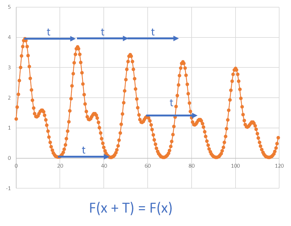Figure 1. Periodic function

Real biological data are rarely perfectly represented by mathematical curves. Time series data, which are measurements taken over time to depict cyclical biological processes such as circadian rhythms, often contain noise, damping effects, or underlying trends (Figure 2).

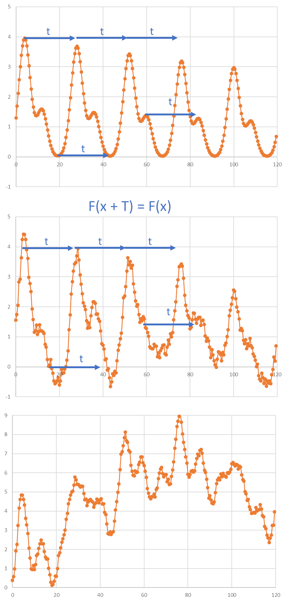
Figure 2. The real biological data typically contains noise as well as trends

In the context of time series data and circadian rhythms, a period refers to the length of time it takes for a repeating pattern or cycle to occur. Specifically, it represents the duration of one complete oscillation or cycle in a cyclical phenomenon. For circadian rhythms, which have a roughly 24-hour period, the period refers to the time it takes for the rhythm to complete one full cycle, typically from one peak (or trough) to the next peak (or trough).

In order to characterize the data with period/phase/amplitude we model the observed signal as known mathematical function of periodic properties, typically cosine.

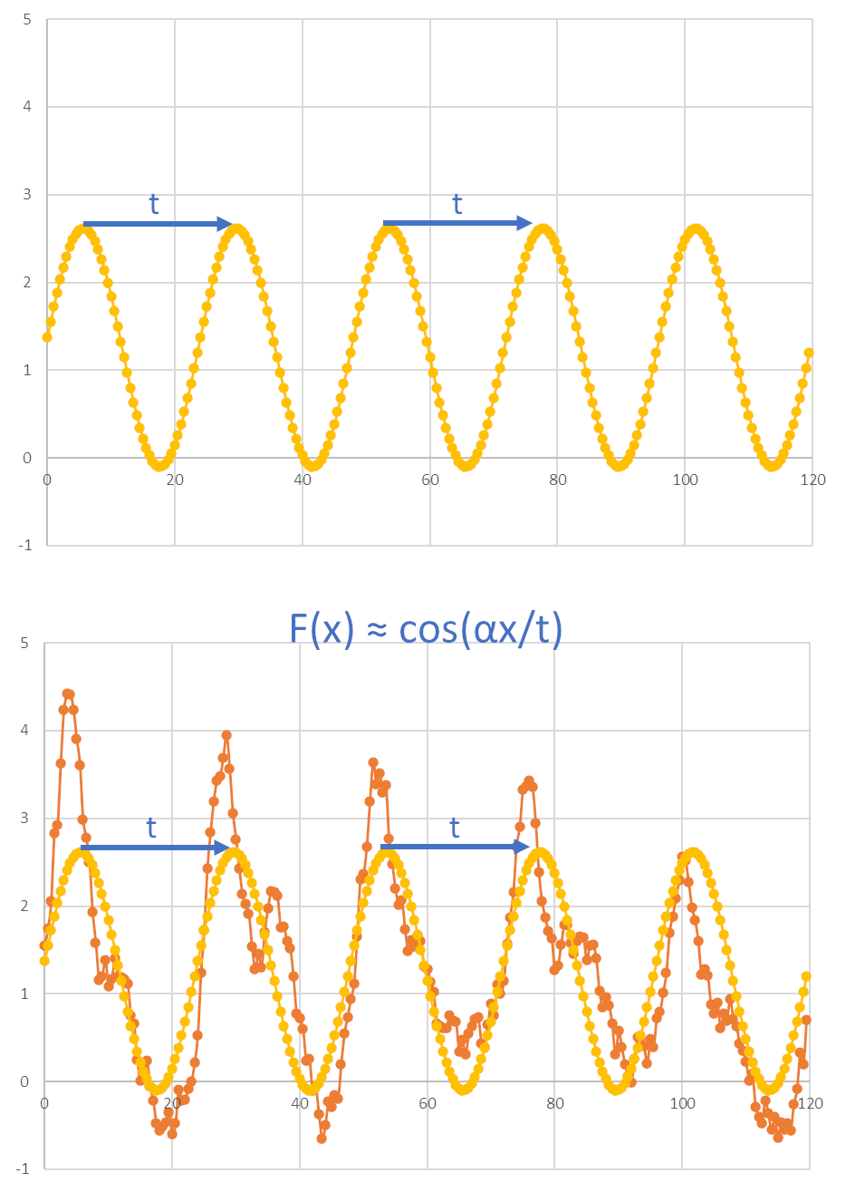
Figure 3. Modelling data with a periodic function

Curve fitting

Curve fitting, also known as regression analysis, is a statistical technique used to find the best-fitting curve or function that describes the relationship between variables in a dataset. The goal of curve fitting is to identify the mathematical model that most accurately represents the pattern or trend observed in the data.

The first step is to choose a mathematical model or equation that is believed to represent the relationship between the variables in the dataset. Common models include linear or polynomial for trends and sinusoidal functions for oscillations.

Once a model is selected, the next step is to estimate the parameters of the model that best fit the data. These parameters are the coefficients or constants in the mathematical equation that determine the shape and position of the curve.

For trends it will be the slope aand intercept b in the trend y = ax + b

For cosine it will be its period, phase and amplitude:

f(x)=A cos(2π/T * ​(x−P)) where T is period, P is phase and A amplitude.

Curve fitting aims to minimize the difference between the observed data points and the values predicted by the model. This is typically done by minimizing a measure of the residuals, such as the sum of squared differences between the observed and predicted values (least squares method).

It turns out that all “decent” functions (signals) can be reconstructed as a sum of various cosine components of different phase, period and amplitude. While the exact reconstruction may involve a very large number of components (in theory indefinite), using only 5 cosine components we can obtain quite complex shapes (Figure 4).

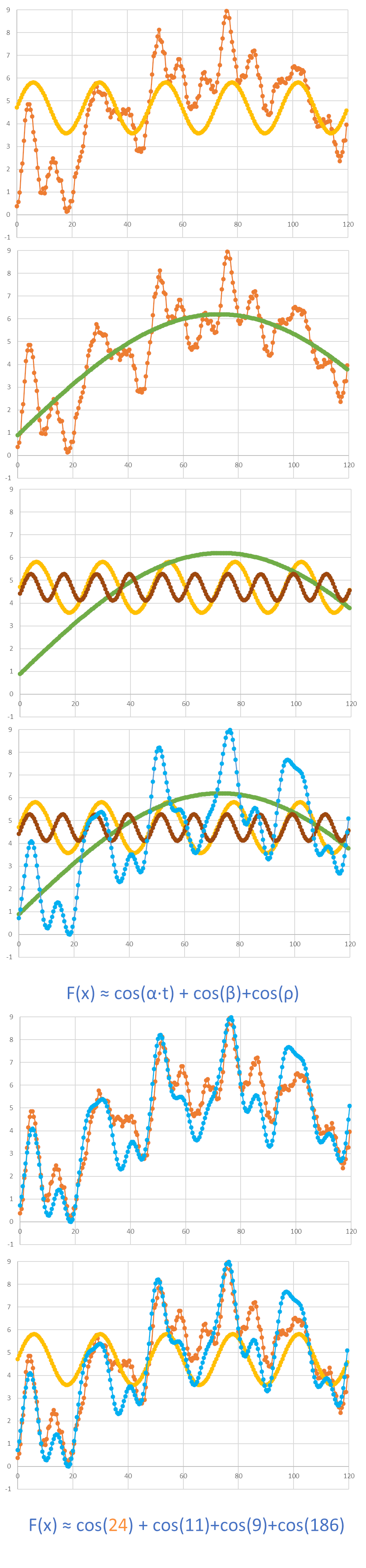Figure 4. Modelling data as a sum of cosines.

We select properties of the either:

• the main consine component i.e. with a larger amplitude
• the circadian component, i.e. with period within sensible range (for example 20-28 hours)

Phase

In circadian data analysis, the phase typically refers to the timing or position of a specific event or feature within the circadian cycle. It indicates where in the cycle a particular biological process or rhythm reaches a certain point, such as a peak, trough, or critical transition.

In the context of a cosine function, the phase represents the horizontal shift (to the right or left) of the cosine curve along the x-axis.

For a standard cosine function f(x)=cos⁡(x), the phase is typically considered to be zero, meaning the curve starts at its maximum value at x=0 and proceeds from there.

However, in the more general form of a cosine function with a phase shift, represented by
f(x) = A * cos(2π/T * (x - P))
the phase shift P determines where along the x-axis the cosine curve starts.

If P>0, the curve is shifted to the right, meaning it starts its oscillation later than the standard cosine function.

If P<0, the curve is shifted to the left, meaning it starts its oscillation earlier than the standard cosine function.

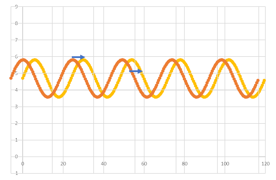
Figure 5. Phase shift of cosine

For biological data we do not know the “original” shape which is being shifted py a phase. So we do a mental jump and use a marker positions (for example peak) relative to a reference point (for example dawn).

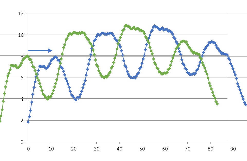
Figure 6. Phase shift of unknown function

In practice we could use following metrics to define phase

• position of the first peak in the original data
• position of the first peak in the smoothed data (better)
• circular average position of peaks (we need to know the period of the signal, to get peaks in each period-wide window)
• we can fit a cosine function and use its phase

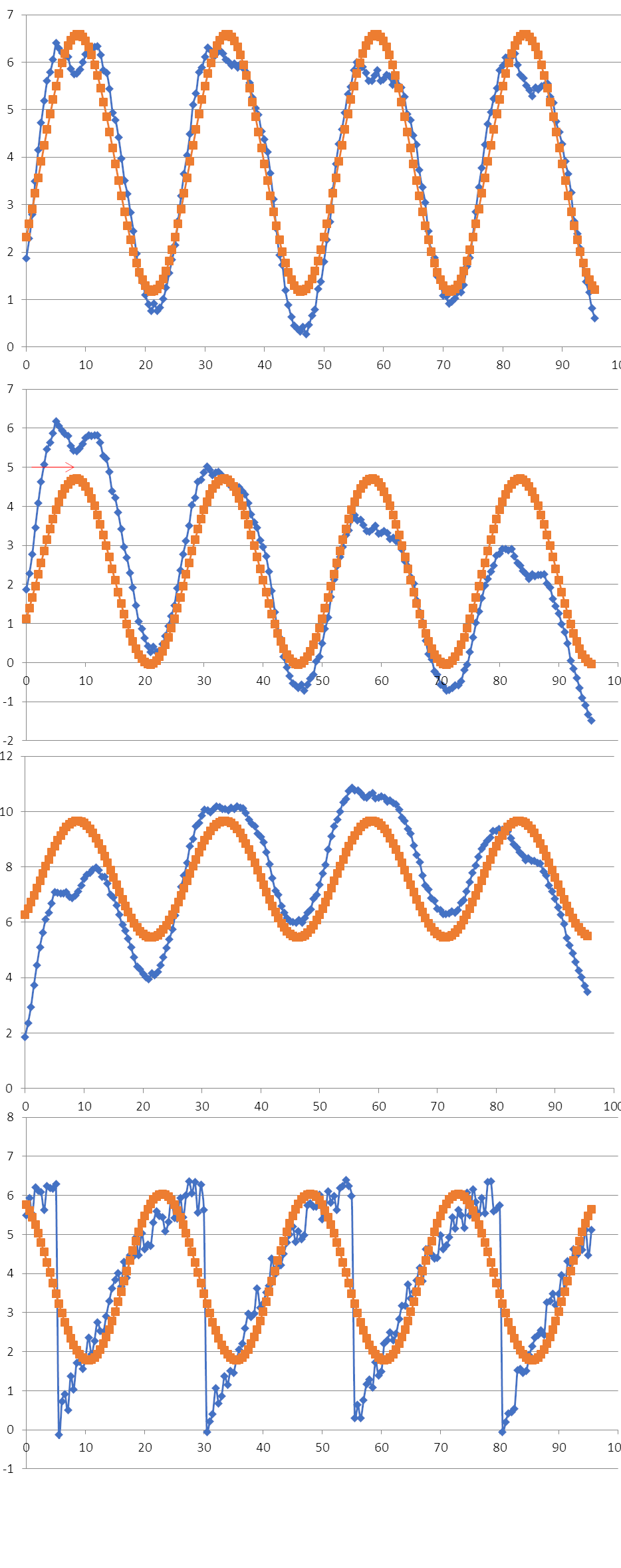
Figure 7. Phase by fitting cosine

As can be seen in the bottom graph of Figure 7, the cosine fit is not a perfect introduces bias if the signal is not symmetrical, in the sense that it does not coincide with the peak time.

Finally, in the circadian field we may prefer using other measures, like onset/offset of activity to define the daily timing of the events (Figure 8).

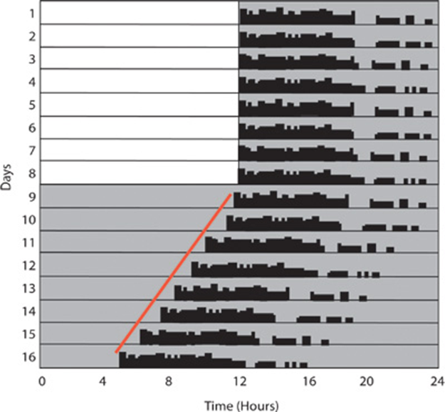
Figure 8. Onset of activity. Credit http://dx.doi.org/10.3791/2463

Methods

Cosinor - originally fit one cosine of period 24h to the data.

Fitting f(x) = A * cos(2π/T * (x - P)) is easy if we know the period T. In that case, the cosine of phase P, is equivalent to a sum of cos and sin with the same period but different amplitudes.
A * cos(2π/T * (x - P)) = α *cos(2π/T * x) - β * cos(2π/T * x)

as both the T is known and the x (x is the time of each measurement/data point), α β can be found by simple linear regression. The original phase and amplitude can be computed using the ratio of alpha and beta values.

That works for the entrained (to 24h) data, but, what to do for free running periods. We can scan circadian period range, for example between 20 and 28 hours every hour. We can then fit a cosine of this period to the data, and select the one period which had the smallest error in the fit.

MFourFit - tries to reconstruct the signal using harmonics.

It takes main cos and sin of a given period T and adds to them up to 5 harmonics, ie. it adds cos and sin of periods T/2 T/3 T/4 T/5. It is a simple linear regression problem. Once the components are found it calculates the fit error.

As you could probably guess, to get the period values, it scans periods within an interesting range and selects the one for which the best fit could be obtain.

FFT NLLS - this method is also based on curve fitting, but, unlike the previous one it simultaneously fits period and phase and amplitude. It is possible using computational intensive non-linear least square method.

It finds up to 5 cosine (typically 3 is enough) components of different phase, period and amplitudes which summed estimate the original curve. The properties of the cosine component of period within the circadian range are used as the period, phase, and amplitude.

The non linear fitting requires sensible starting period parameters to succeed, to find those initial guesses the FFT method is used. Hence, the name FFT NLLS. Fast fourier transform calculates the main frequency components in the signal (frequency is 1/T).

So why the FFT alone is not used instead? The frequency resolution of fft (so which peaks can be found) depends on number of data points and the interval between them, and in typical circadian data is not good enough to distinguish for example between periods 24 and 23h.

Maximum Entropy Spectral Analysis (MESA) - uses a completely different approach based on stochastic modelling. MESA first fits an autoregressive model to the data. This model assumes that the value at a given time point is the combination of a number of previous values plus some stochastic process (noise):

X[t] = a1X[t-1]+ a2X[t-2]+ a3X[t-3]+ …+anX[t-N]+ η

(where: ai are model coefficients, X[t-i] is the data value at previous time point t-i, η is noise, N is the length of the model)

Model coefficients can also be considered as the coefficients of a prediction filter (PF) of length N, where the next value can be predicted using the previous values. Such equations can be written for each data point and filter coefficients that minimise the difference between the predicted and original values can be found using a least-squares approach.

It is possible to obtain a frequency spectrum for the data by using the prediction coefficients. In general, a frequency spectrum characterizes the presence (contribution) of each frequency within the signal, with the most common example being the Fourier Transform power spectrum. Since frequency is the inverse of the period, finding the maximum in a frequency spectrum also identifies the strongest period of the data.

More information on period analysis

BioDare2 docs
Comparison of period analysis methods

Quiz

Answer True / False to the following statements.

• there is one and clear definition of phase in circadian data
• all methods of period analysis are based on fitting cosine curves
• using time of peaks can be used to describe phase of the data
• using time of troughs can be used to describe phase of the data
• cosine function is the best model for periodic signals

Solution

• there is one and clear definition of phase in circadian data (False)
• all methods of period analysis are based on fitting cosine curves (False, MESA, periodograms are example of methods without curve fitting)
• using time of peaks can be used to describe phase of the data (True)
• using time of troughs can be used to describe phase of the data (True)
• cosine function is the best model for periodic signals (False, it depends on the shape of the signal, a square pulse may be better for activity data)

Key Points

• There is no one best period analysis methods, the performance depends on duration, sampling and noise level of the data